Uncertainties, As I Understand It

Uncertainties, As I Understand It 2 December 2019

This will be the first in I hope a series of posts about me writing down something as I understand it. The point of this is to help me get it straight in my head, but also admit where I don’t know things. I am wrong in many regards, and these will most likely be some of the many times that I am.

Since this also serves as an introduction of sorts if someone happens to read this (unlikely) who also happens to be able to correct me / help me, contact information is on the about page.

An Introduction of Sorts

When performing a measurement, you (usually) get a single value. However it is impossible to be certain that the value you get is the absolute correct value. So you give a range of values that it could be in.

Typically you give a standard deviation along with the value. These quantities I write as (1.0 ± 0.1) m. However some other notations exist, and are used. I won’t cover them here because I am far too lazy to write about it.

A Visual Description

I will show here some real data that I gathered in one of my lab sessions, it represents a very very bad scan with an AFM (atomic force microscope~~(microscopy?)~~). I say very bad and I mean it. Specifically it represents the height data.

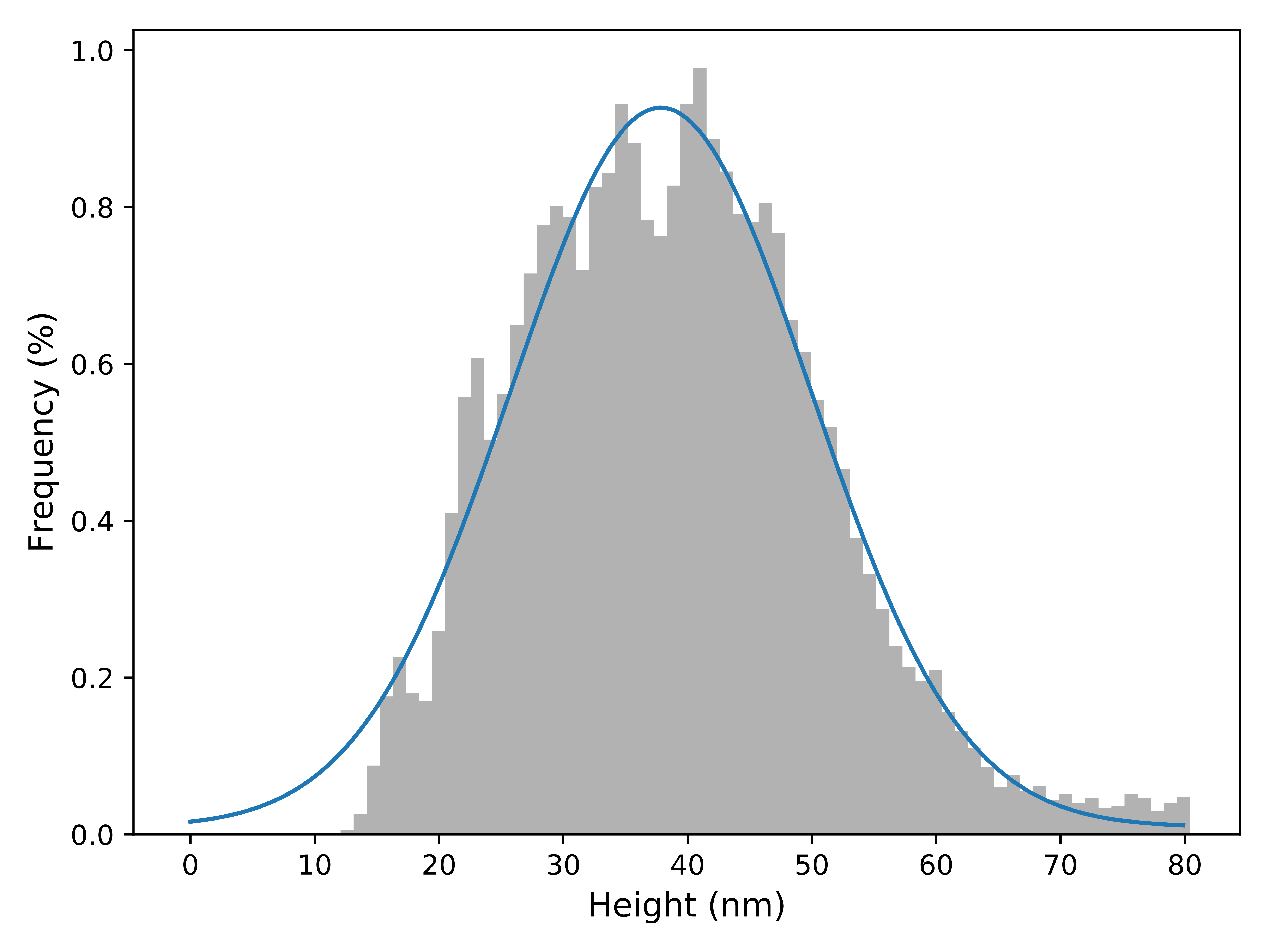
Some real data gathered using an AFM. This shows a histogram of the height profile.

Simply by looking at the graph, and the fit, you can see that I can quantify how close I think the “actual” value is to the peak. And since I rather conveniently used a Normal/Gaussian/Whatever fit, I can very easily get the standard deviation that I so crave.

How to actually use these things

Once you have a value and an uncertainty, you might want to combine these with some other values. The derivations are not that hard, but often someone’s already derived them for you.

The Wikipedia article on uncertainty propagation contains some examples of these formula, as well as derivations.

The basic result of this is what is apparently known as the “variance formula”.

\sigma_f^2 = \left(\frac{\partial f}{\partial x}\right)^2 \sigma_x^2 + \left(\frac{\partial f}{\partial y}\right)^2 \sigma_y^2 + \cdots

The Wikipedia article has it written with a square root on both sides, but I think this looks a maybe better. Anyway, if you have some function $f(x, y) = \sin(x) + \cos(y)$ then the standard deviation in the function can be calculated by

\begin{aligned} \sigma_f^2 &= \left(\frac{\partial f}{\partial x}\right)^2 \sigma_x^2 + \left(\frac{\partial f}{\partial y}\right)^2 \sigma_y^2 \\ &= \cos^2(x) \sigma_x^2 + \sin^2(y) \sigma_y^2 \end{aligned}

Simple?

Fun with this

I think that it is possible to do this sort of thing with numerical differentiation, rather than symbolic differentiation. Therefore given some arbitrary function and some values with uncertainties it should be possible to come up with how they combine using the function provided. I might give this a go at some point using what I learned from the performing regressions to arbitrary functions with scipy.

Edit 2019-12-03: I have now done this. You can find it on my GitHub.

Wrap up

Again, comments or corrections to the address in the about page.